Project 4: Neural Radiance Field!
[View Assignment]Part 0: Camera Calibration and 3D Scanning
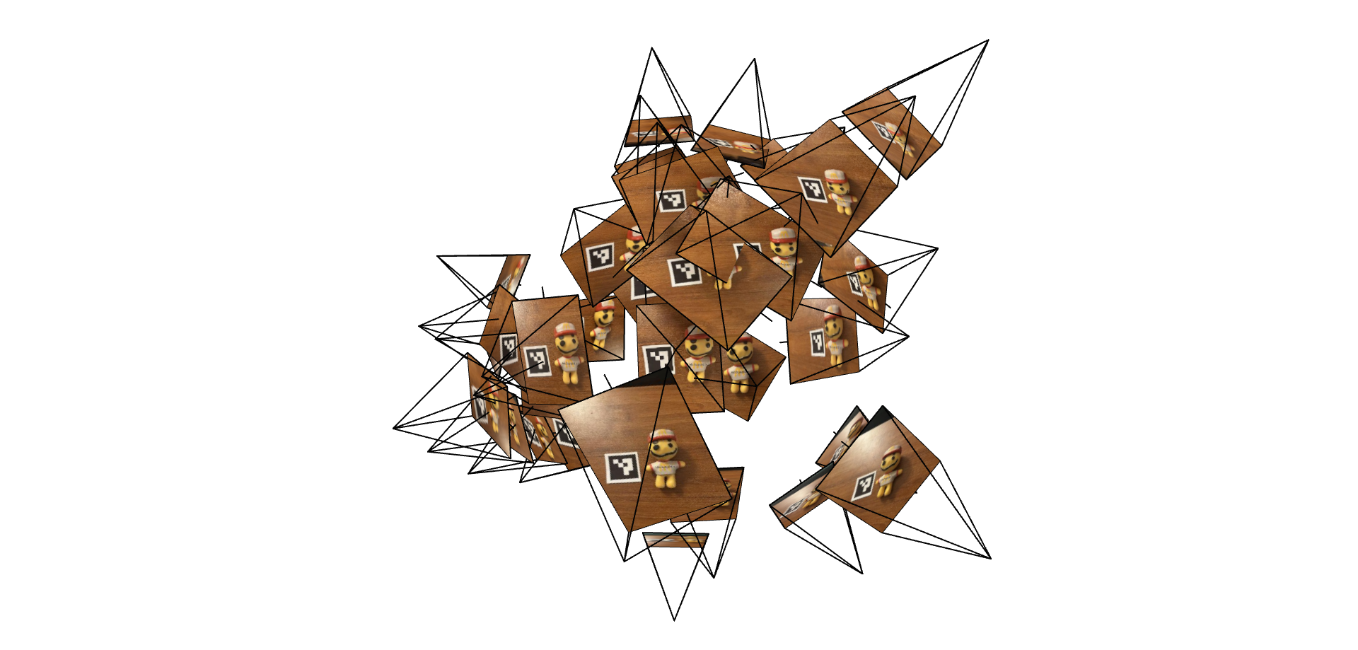
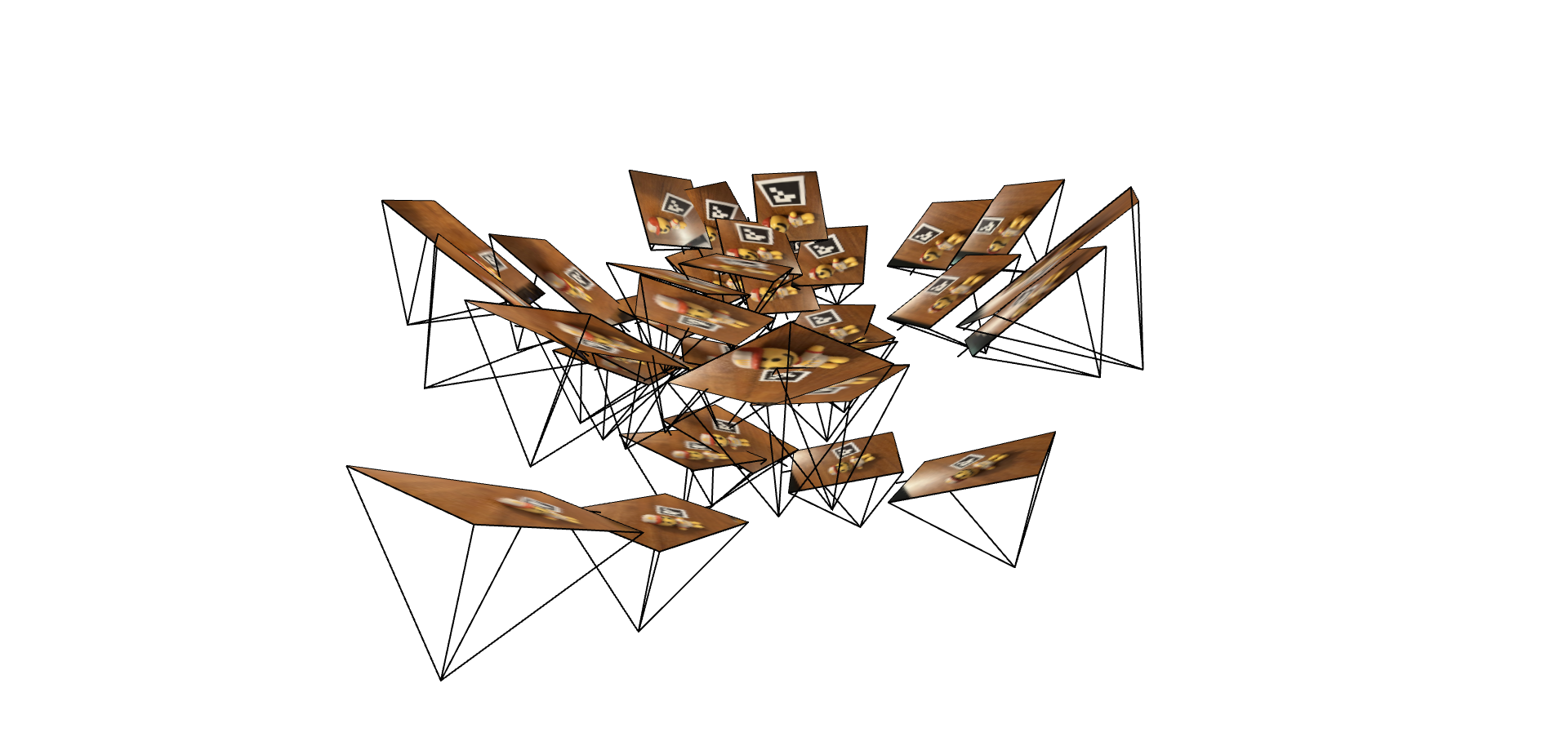
For this part, I took a 3D scan of my own object using ArUco tags to first calibrate my camera parameters, then using them to estimate the camera pose for each image of my object. Aftwards, I undistorted my images and packaged them with the instrinsics into a dataset that will be used create a NeRF later on. There were 40 total images, with 36 being valid to use.
Part 1: Fit a Neural Field to a 2D Image
I created a Neural Field that can represent a 2D image and optimize it to fit two different images.
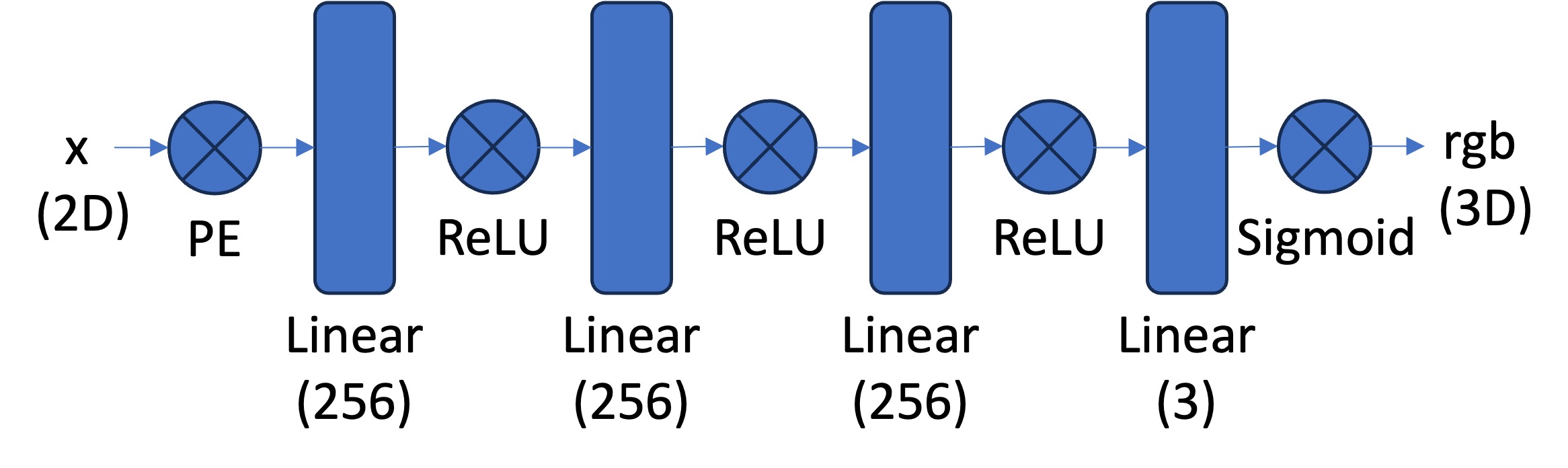
The model architecture first inputs a two-dimensional pixel coordinate \((u, v)\) into a sinusoidal positional encoder (PE) to expand its dimensionality (the reconstruction below uses \(L=10\) frequencies per pixel, i.e., it maps the 2D coordinate to a 42D vector). This is then fed into a multilayer perceptron (MLP), which uses four linear layers of width 256, with the first three being followed by a ReLU activation layer, and the last layer being followed by a Sigmoid activation layer to output the three-dimensional \((r, g, b)\). Below is a visualization of the network:
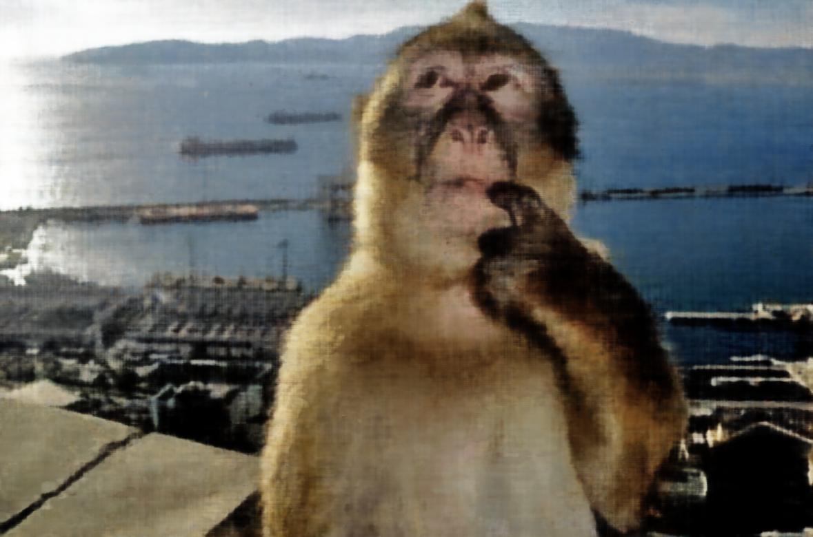
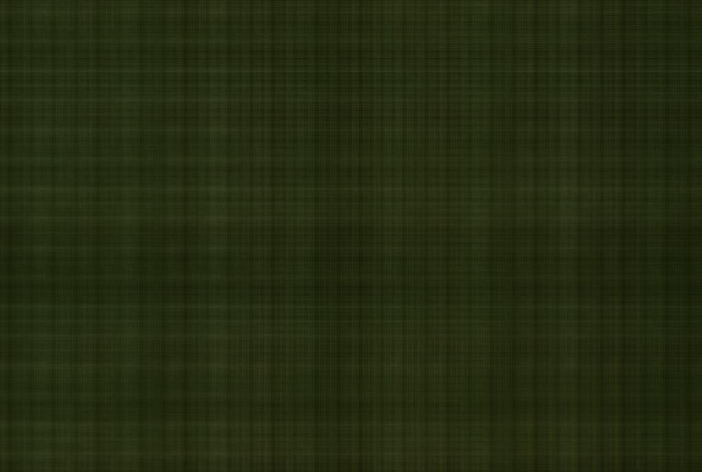
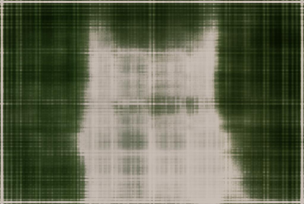
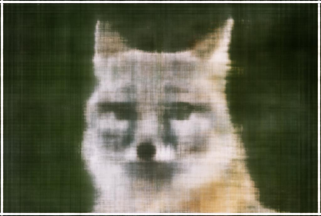
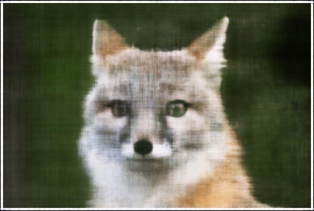
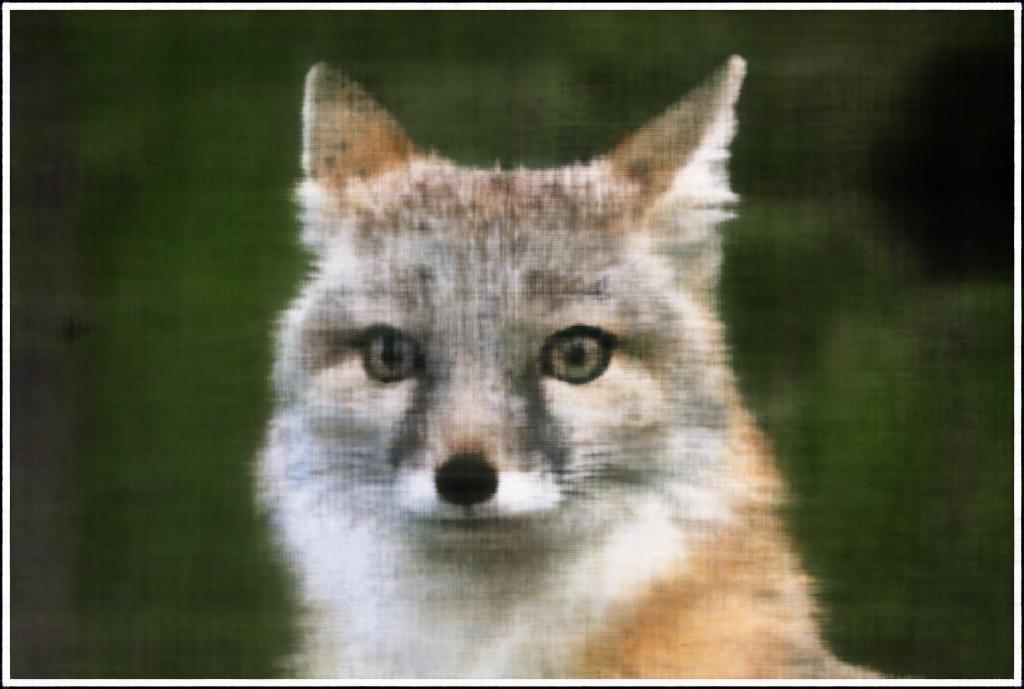
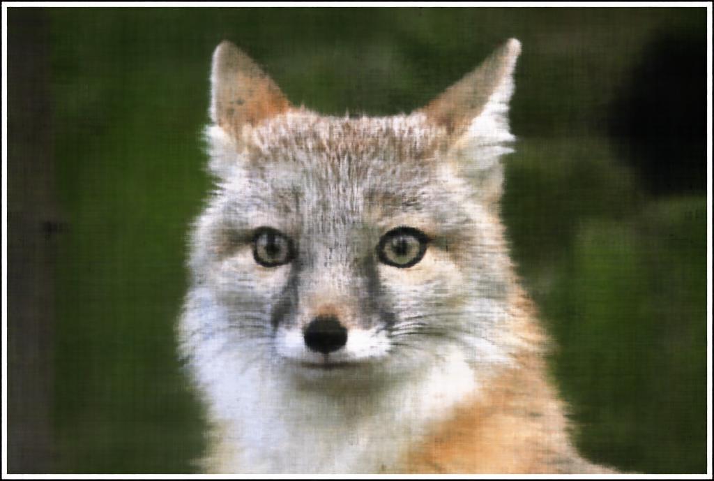
These are the training progression of two different images over 2000 iterations. I used an Adam optimizer with a learning rate of \(0.01\) to train the network.

1
50
100
200
500
2000
1
50
100
200
500
2000
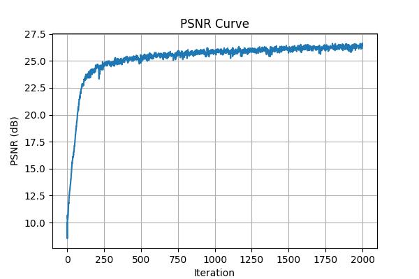
Training PSNR curve on fox image.
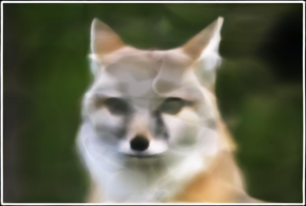
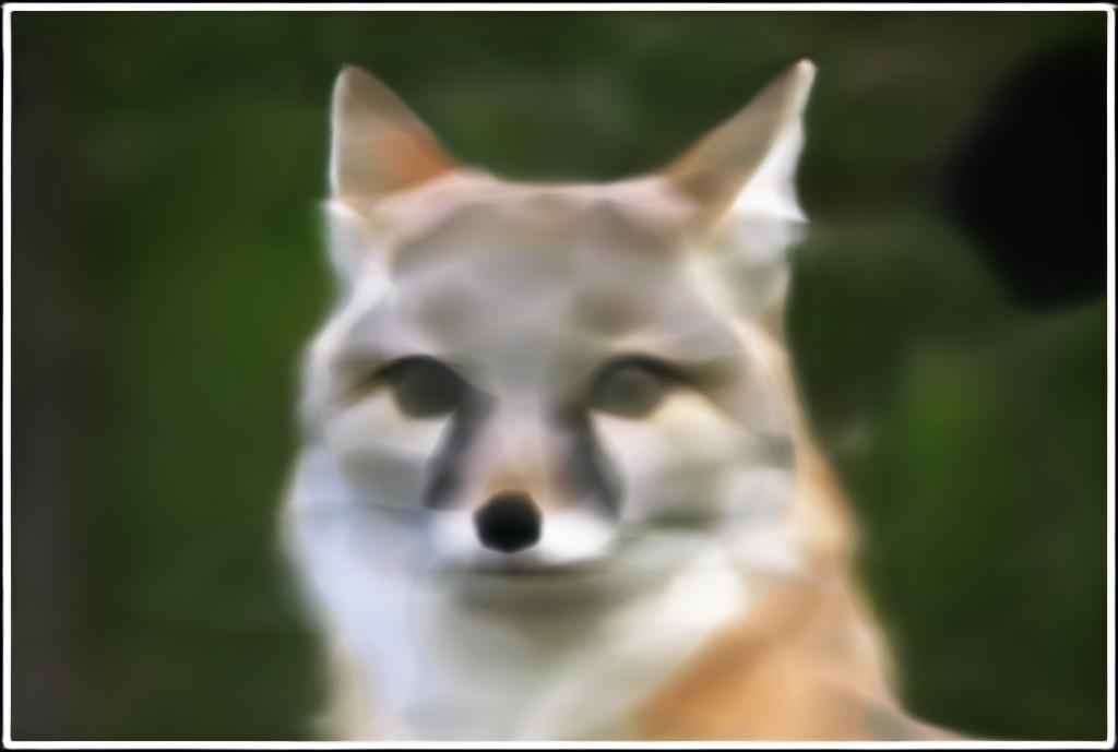
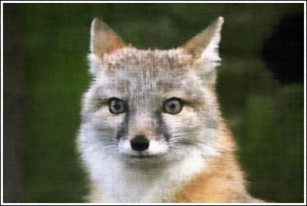

With a low max frequency (\(L = 3\)), the positional encoding captures only low-frequency structure, so the Neural Field produces smoother and blurrier outputs. Increasing to \(L = 15\) adds high-frequency detail, giving sharper renderings when the network width is moderate (e.g., 128). But combining high frequency (\(L = 15\)) with a large width (512) makes the network unstable: activations and densities grow too large, the volume-rendering weights collapse, and the output becomes entirely black.
Part 2: Fit a Neural Radiance Field from Multi-view Images
Part 2.1: Create Rays from Cameras
Camera to World Coordinate Conversion
The transformation between the world space and the camera space, which is defined by the world-to-camera transformation (extrinsic) matrix, \(\text{w2c} = \begin{bmatrix} \mathbf{R}_{3\times3} & \mathbf{t} \\ \mathbf{0}_{1\times3} & 1 \end{bmatrix}\), is:
\(\begin{align} \begin{bmatrix} x_c \\ y_c \\ z_c \\ 1 \end{bmatrix} = \begin{bmatrix} \mathbf{R}_{3\times3} & \mathbf{t} \\ \mathbf{0}_{1\times3} & 1 \end{bmatrix} \begin{bmatrix} x_w \\ y_w \\ z_w \\ 1 \end{bmatrix} \end{align}\)
The inverse of the extrinsic matrix \(\text{w2c}\) is called the camera-to-world transformation matrix \(\text{c2w}\). I implemented a function X_w = transform(c2w, X_c) that uses the \(\text{c2w}\) matrix to transform a point from camera \(\mathbf{X_c} = \begin{bmatrix} x_c & y_c & z_c \end{bmatrix}^\top \) to world space \(\mathbf{X_w} = \begin{bmatrix} x_w & y_w & z_w \end{bmatrix}^\top\).
Each camera-space point \(\mathbf{X_c}\) is augmented with a homogeneous coordinate (by appending 1) to form \(\mathbf{X_{c_h}}= \begin{bmatrix} x_c & y_c & z_c & 1 \end{bmatrix}^\top\). The code then performs a batch matrix multiplication:
x_w_h = torch.bmm(c2w, x_c_h)
The result x_w_h represents the same points expressed in world coordinates \(\mathbf{X_{w_h}}\). After dropping the homogeneous coordinate, I obtained the transformed 3D positions in world-space \(\mathbf{X_w}\).
Pixel to Camera Coordinate Conversion
The transformation between the 2D pixel coordinate system to the camera coordinate system is
\(\begin{align} s \begin{bmatrix} u \\ v \\ 1 \end{bmatrix} = \mathbf{K} \begin{bmatrix} x_c \\ y_c \\ z_c \end{bmatrix} \end{align}\),
for some intrinsic matrix
\(\begin{align} \mathbf{K} = \begin{bmatrix} f_x & 0 & o_x \\ 0 & f_y & o_y \\ 0 & 0 & 1 \end{bmatrix} \end{align}\),
X_c = pixel_to_camera(K, uv, s) that uses the intrinsic matrix \(\mathbf{K}\) to transform a pixel coordinate \(\begin{bmatrix} u & v \end{bmatrix}^\top\) with a given depth value \(s\) to a camera-space coordinate \(\mathbf{X_c} = \begin{bmatrix} x_c & y_c & z_c \end{bmatrix}^\top\).
The homogeneous pixel coordinates \(\begin{bmatrix} u & v & 1 \end{bmatrix}^\top\) are multiplied by the inverse of the intrinsic matrix \(\mathbf{K}^{-1}\):
x_c = torch.bmm(K_inv, uv_h)
This yields points on the camera plane (in units of depth s) measured along the camera's optical axis. Each pixel now corresponds to a direction vector in camera space pointing away from the camera center.
Pixel to Ray
Finally, I implemented ray_o, ray_d = pixel_to_ray(K, c2w, uv), that utilizes pixel_to_camera and transform to convert a pixel coordinate \(\begin{bmatrix} u & v & 1 \end{bmatrix}^\top\) to a ray with an origin vector \(\mathbf{r}_o\), which is simply the translation component \(\mathbf{t}\) in the \(\text{c2w}\) transformation matrix, and a normalized direction vector \(\begin{align} \mathbf{r}_d = \frac{\mathbf{X_w} - \mathbf{r}_o}{||\mathbf{X_w} - \mathbf{r}_o||_2} \end{align}\).
Specifically, it first calls pixel_to_camera to convert pixels to camera-space coordinates, then uses transform to convert those to world coordinates. The ray origin ray_o is taken directly from the camera translation component c2w[:, :3, 3], and the ray direction ray_d = (x_w − ray_o) is normalized to unit length:
ray_d = ray_d / torch.norm(ray_d, dim=-1, keepdim=True)
This produces a pair of tensors (ray_o, ray_d) for every pixel, representing the origins and normalized directions of all rays emitted from the camera through the image plane. These rays are later used for sampling along 3D volumes in the NeRF rendering pipeline.
Part 2.2: Sampling
Sampling Rays from Images
I implemented a PyTorch Dataset class, RaysData, to represent all camera rays and corresponding pixel colors across multiple training images. The class encapsulates the relationship between image pixels, camera parameters, and their corresponding world-space rays. It takes as input:
images: a tensor of shape(B, H, W, 3)containing RGB imagesK: the \(3 \times 3\) intrinsic matrixc2ws: the camera-to-world extrinsic matrices for each imagedevice: either"cpu"or"cuda".
Each image pixel color is flattened into a long tensor to do a global ray sampling from all images (use for the sample_rays method). Then a full grid of pixel coordinates \(\begin{bmatrix} u & v \end{bmatrix}^\top\) is generated for every image using torch.meshgrid(), and a +0.5 offset is added to center the ray at the middle of each pixel. These pixel coordinates are then converted into 3D rays using pixel_to_ray, which applies both intrinsic and extrinsic transformations to produce the ray origin and normalized ray direction vectors. Finally, both are also flattened so each pixel in all images corresponds to one ray.
The RaysData class contains these methods:
sample_rays(N): selects \(N\) random rays from the total set, returning their origins, directions, and ground-truth pixel colorssample_rays_from_one_image(): randomly selects one full image and returns all rays and pixels from that view; mainly used for generating novel view reconstructions or evaluation renderingsget_rays_from_c2w(c2w): generates rays for any new camera posec2w, as it constructs pixel grids for that image and usespixel_to_ray()to map them to world-space rays; used for rendering test or synthetic views (e.g., orbiting around the object).
Sampling Points along Rays
I then implemented sample_along_rays to generate 3D sample points along each ray between the near and far bounds. This function creates evenly spaced 3D sample points along each ray between the near and far clipping planes. It defines a set of depth values t between near and far using torch.linspace(near, far, n_samples).
If perturb=True, random noise is added to t to introduce jitter for stratified sampling, improving rendering smoothness:
t = t + torch.rand(t.shape) * (far - near) / n_samples
Then each 3D coordinate is then computed as
\(\begin{align} \mathbf{x} = \mathbf{R}_o + \mathbf{R}_d * t \end{align}\),
This yields a tensor of shape (N, n_samples, 3) containing all the sample positions along each ray, which are later passed through the NeRF model to predict color and density values.
Part 2.3: Putting the Dataloading All Together
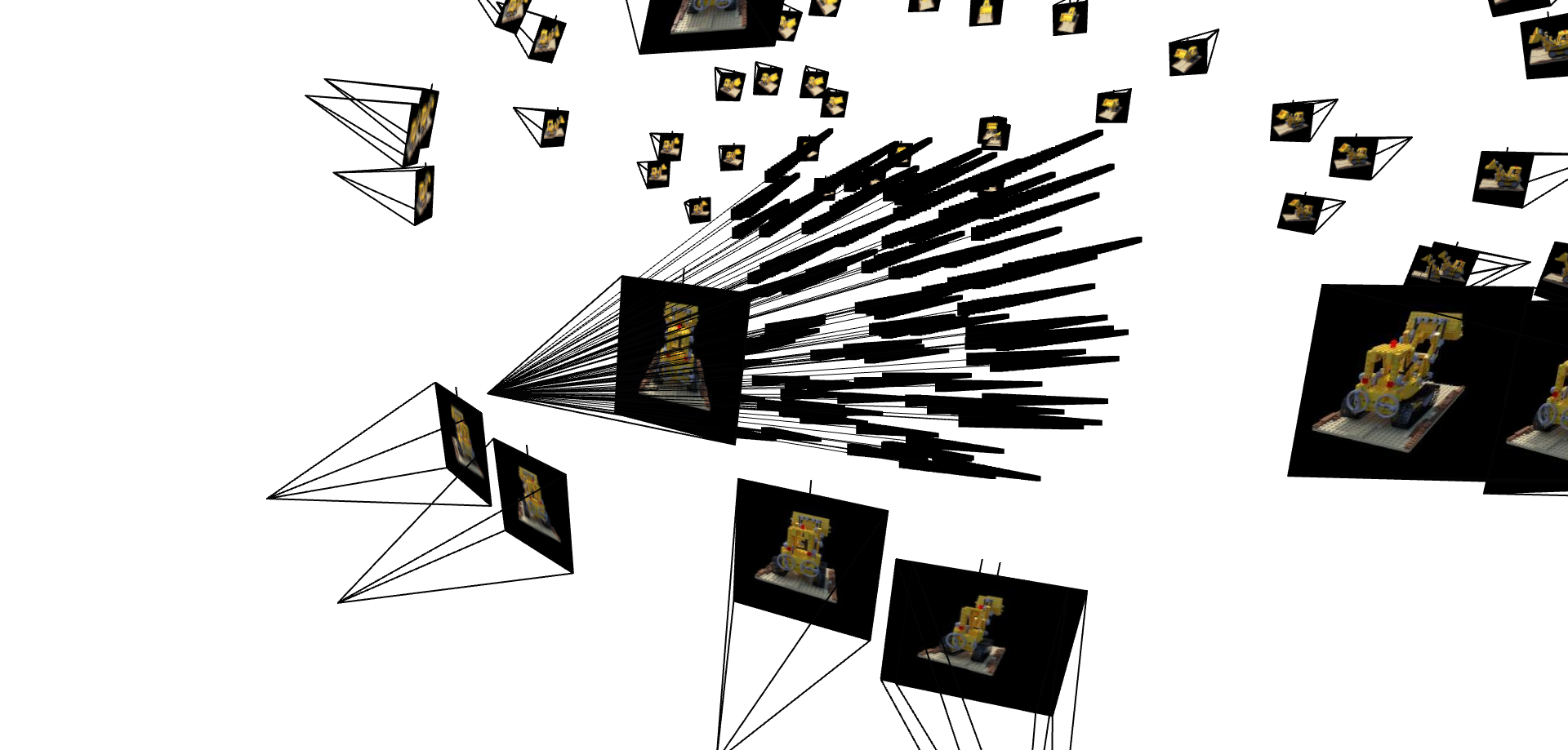
Using the provided visualization code, I plotted the cameras, rays, and samples in 3D of the lego dataset to verify that Part 2.1 and 2.2 have been done correctly.
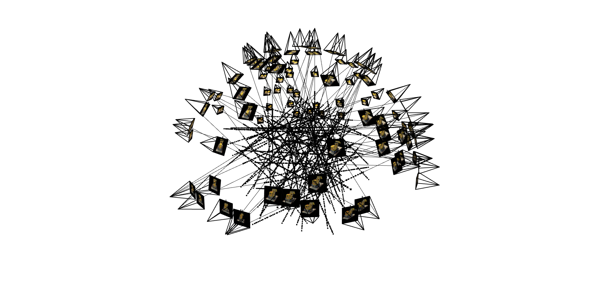
Rays sampled from every camera.
Rays sampled from one camera.
Part 2.4: Neural Radiance Field
To create the NeRF, using the same ideas to the MLP in Part 1, I first implemented a deeper MLP, NeuralRadianceField, to predict the density and color of the sampled 3D points on the rays. Below is a visualization of the network:
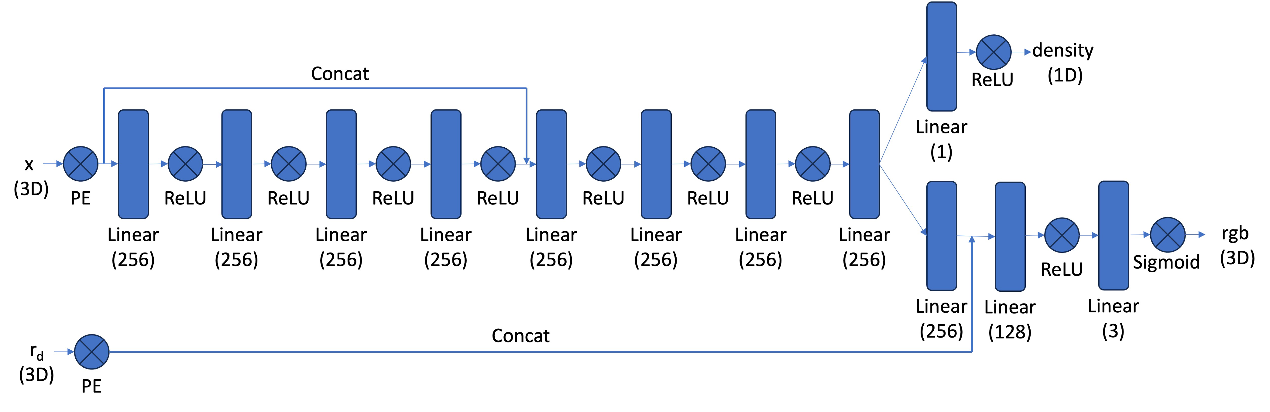
The NeuralRadianceField model uses positional encoding to map both 3D coordinates and ray directions into a higher-dimensional space, allowing the network to learn high-frequency details.
Two separate encoders (coord_pe and ray_d_pe) are applied before passing the inputs through multiple MLP blocks.
The first MLP block (mlp_block1) extracts spatial features from the encoded 3D positions, while the second block (mlp_block2) refines them after concatenation with the original positional encoding.
The network then branches into two outputs:
- Density (\(\sigma\)): predicted by
density_layer, representing the volume density of each point along the ray. - Color (RGB): predicted by
rgb_layer_block1andrgb_layer_block2, which combine spatial features with the encoded ray direction.
This architecture allows the model to represent a continuous volumetric field that can synthesize novel views of the scene by integrating colors and densities along sampled rays.
Part 2.5: Volume Rendering
After the MLP outputs the color (RGB) and density (\(\sigma\)), the NeRF renders the color using the volume rendering equation:
\(\begin{align} C(\mathbf{r})=\int_{t_n}^{t_f} T(t) \sigma(\mathbf{r}(t)) \mathbf{c}(\mathbf{r}(t), \mathbf{d}) d t, \text { where } T(t)=\exp \left(-\int_{t_n}^t \sigma(\mathbf{r}(s)) d s\right) \end{align}\)
I implemented the discrete appromixation of it,
\(\begin{align} \hat{C}(\mathbf{r})=\sum_{i=1}^N T_i\left(1-\exp \left(-\sigma_i \delta_i\right)\right) \mathbf{c}_i, \text { where } T_i=\exp\left(-\sum_{j=1}^{i-1} \sigma_j \delta_j\right) \end{align}\),
for a batch of samples along a ray, as volrend(sigmas, rgbs, step_size). In the implementation, sigmas represents the predicted densities and rgbs the corresponding colors for each sampled point along a ray. The function first converts densities into alpha values using the relation alpha = 1 - exp(-sigma * step_size), which represents the probability of light being absorbed at each sample.
Next, cumulative transmittance T_i is computed using a running product of (1 - alpha) via torch.cumprod(), ensuring that each point's contribution accounts for how much light has been absorbed before reaching it. The element-wise product of T_i and alpha gives the sample weights.
Finally, the rendered color for each ray is obtained by summing the weighted colors along the ray:
rendered_colors = torch.sum(weights * rgbs, dim=1)
This produces the final pixel color, effectively simulating how light accumulates through a semi-transparent volume.
Putting all of this together, I fed the lego dataset into the NeRF. Below are the training progression over 3000 iterations of one of the cameras. Again, I used an Adam optimizer with a learning rate of \(0.0005\) to train the network.

1

50
100
200

1000
3000
Validation PSNR curve on the lego.
After training the network, I created a rendering of the lego from arbitrary camera extrinsics (c2ws_test provided in the .npz file).
Part 2.6: Training with My Own Data
Now I created a NeRF using the dataset I generated in Part 0. I trained a NeRF with these parameters:
- Number of samples per ray: 96
- Number of iterations: 3000
- Batch size: 10000
- Near plane: 0.02
- Far plane: 0.5
- Learning rate: 0.0005
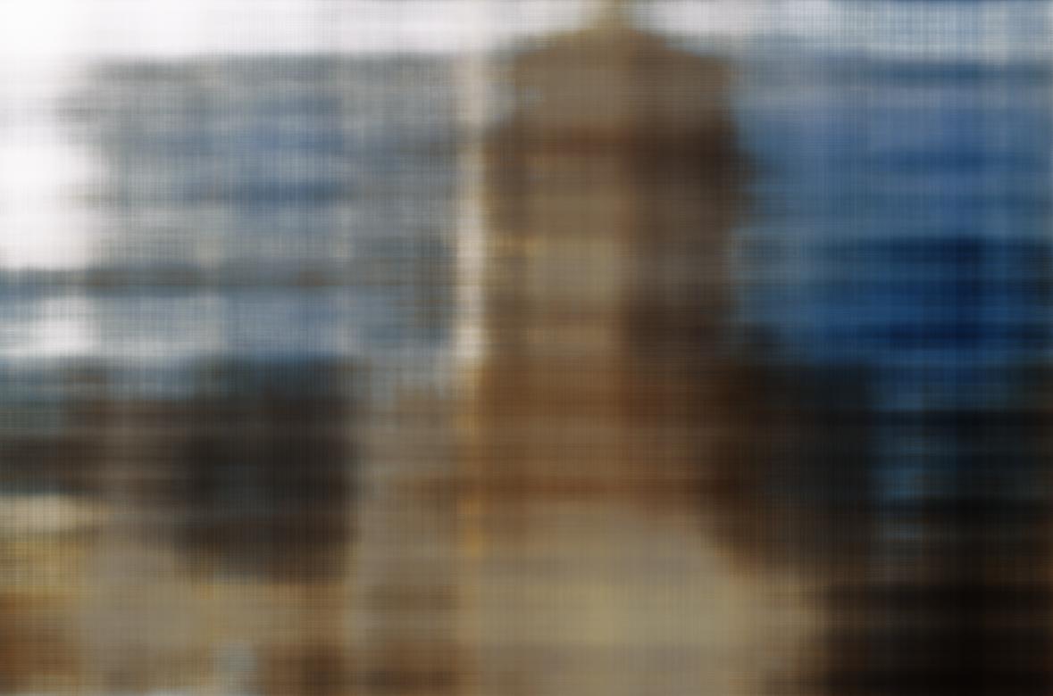
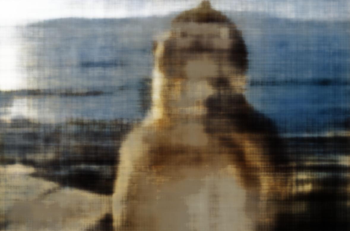
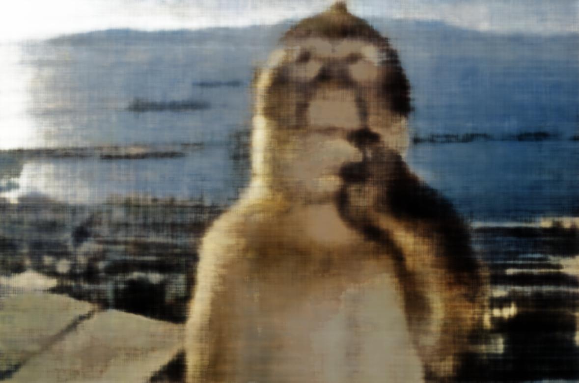
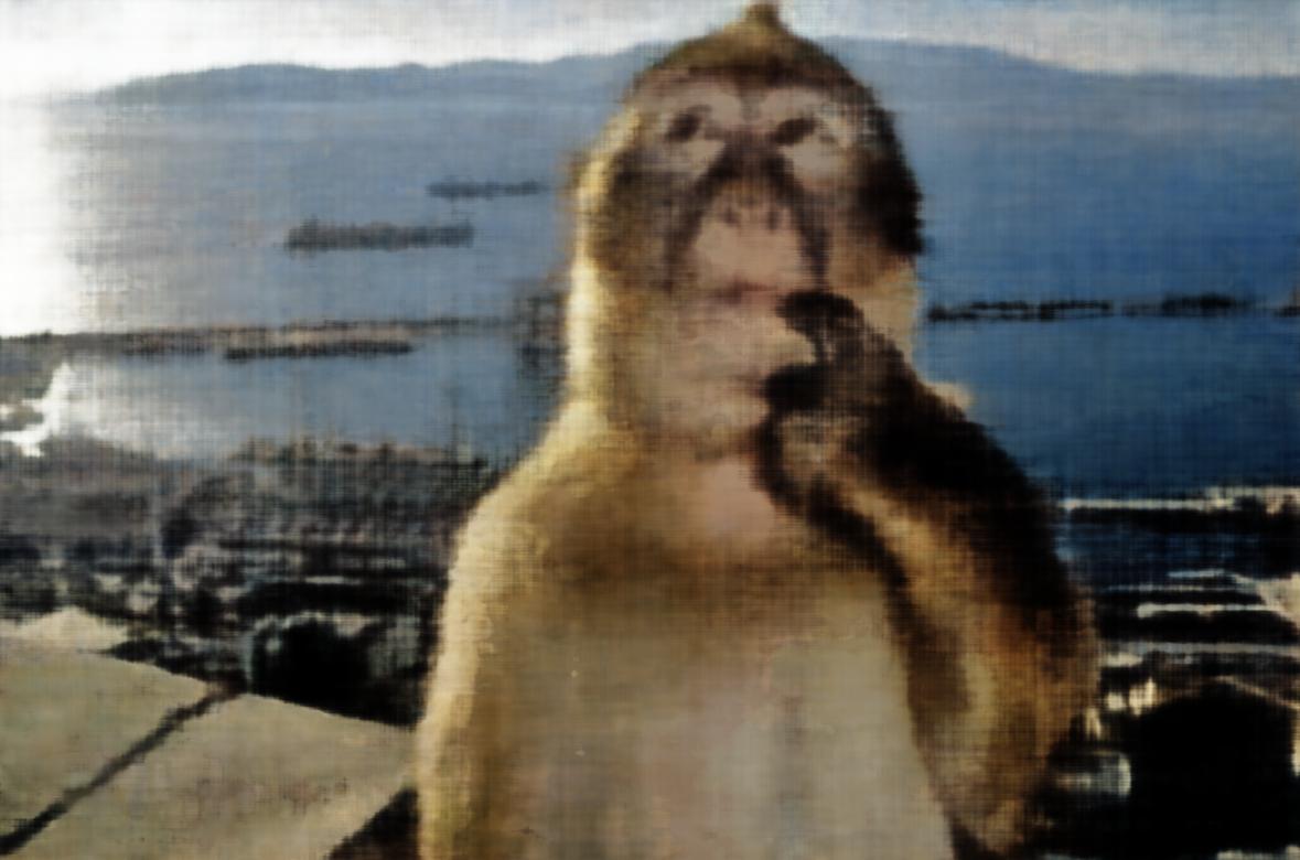
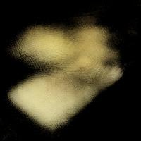
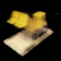
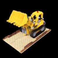
The MLP architecture used is the same. I kept all the previous hyperparameters the same as I did for the lego dataset, but decreased the sampling rate per ray to \(96\) in hopes it would produce a better reconstruction. Here is the training progression over 3000 iterations of one of the cameras.
223
334

667
1000
2000
3000
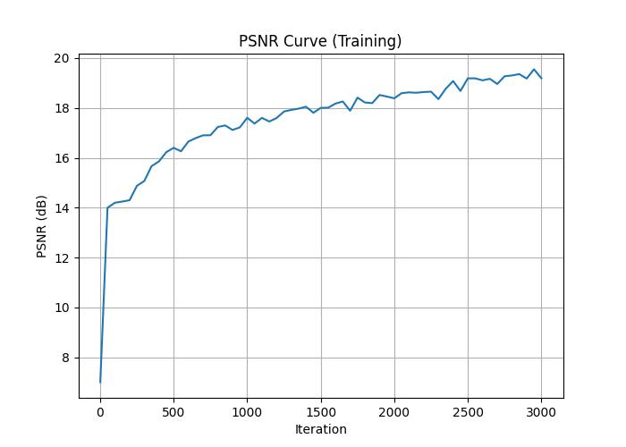
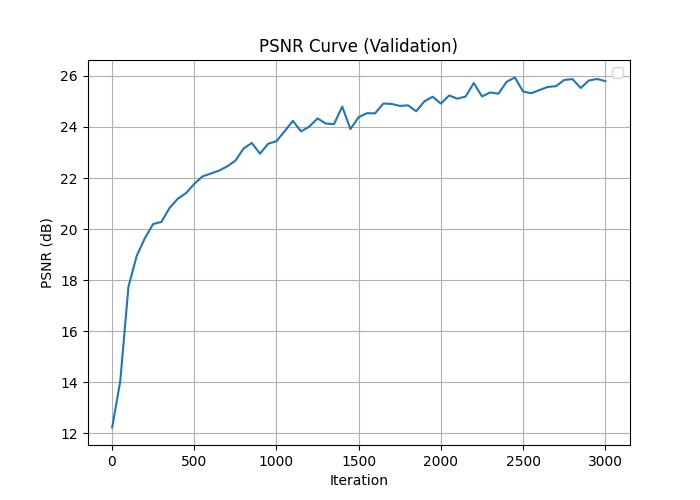
Training PSNR curve on my object.
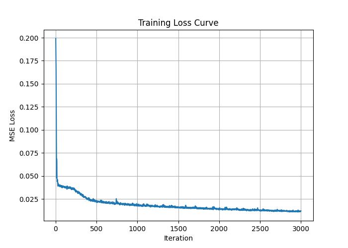
Training loss on my object.
After training the network, I used my test camera extrinsic (from my dataset as c2ws_test) to generate 60 synthetic views rotating around my object to create a 3D rendering. Here is the result: